Category: Skills
-

#12: How To Make Reading Your Research Superpower
A review of research literature is a useful thing to do. It helps us understand what the current thinking, developments and practices are with regard to a particular subject area.
The process of creating the review helps us learn about a topic and it also draws out our opinions as we digest and compare the articles that we discover.
As a product in itself, the review assists other to do research as it brings together thinking about a range of articles into one document. If you want to quickly learn about a subject that is new to you, you should look for literature reviews that have already been completed.
It is common for a literature review to identify challenges for the research at the time of writing. These challenges can help you identify where your contribution to knowledge might lie, or at least which areas are worthy of further investigation.
Conducting a review can seem like a monumental task. Reading all of the literature is time consuming, and it is wise not to waste time on irrelevant material.
We can accelerate the process of conducting a review by ensuring that we use specific approaches to reading and comprehending the content of an article, and also being diligent about recording what we do.
Like any research activity, it helps to discuss your ideas and thinking with others; make sure that you talk about your work and your findings to solicit feedback.
SQ3R is an approach to reading that can increase your efficiency when compiling a review.
The original method was proposed by Francis Robinson and can be found here:
Robinson, Francis Pleasant (1978). Effective Study (6th ed.). New York: Harper & Row. ISBN 978-0-06-045521-7.
Alternatively, there are lots of online resources for SQ3R.
There are five steps: survey; question; read; recite and review.
Survey
To start with, resist the temptation to read an article thoroughly, even though it may look interesting. Read the abstract, conclusions and references first. See if there are any interesting conclusions, and if there are, review the rest of the article lightly. Look at headings and sub-headings, figures and tables. This should take no longer than five minutes to complete. You may want to take notes while you do this.
If you realise that the article is out of scope, off-topic, or just does not relate to your intended study, reject it now. Write some notes about why you are rejecting it; they might be useful at some later stage if you discover something else that is relevant.
Question
Using any notes that you might have written from the survey stage, start to pose some questions about the content of the article. You might want more clarity about the particular research method that was used for instance; think about how useful that knowledge might be to your own study. Write these questions down. Again, this should take no longer than a few minutes.
Read
You can now proceed to read the paper in detail. You will find that you already understand the gist of the article, and you are now in a position to digest what has been written and answer your own questions that you posed in the previous stage. You may take longer to complete this activity. In time, you will become quicker.
Retrieve
You shall now attempt to test your comprehension of the article. Without reading the paper, try and answer the questions that you raised, and also try and explain what the paper is about in your own words. Some people prefer to do this out loud, whereas others prefer to write their thoughts down.
You may find that you generate new questions or ideas at this stage. This is good! Write them down and repeat the Read stage to clarify your understanding.
Review
Regularly reviewing what you understand is important for the success of the SQ3R process. When you read a paragraph, a section, or even the entire article, pause and recite the key elements about the article that you understand, together with any thoughts that you have developed as a result of reading the article.
If you have been diligent through this process, you will have recorded both the formal reference (so that you can cite it at a later stage), and also you shall have notes from each of the subsequent steps.
These notes will help you when it comes to compile your review.
SQ3R is a good way of quickly getting to grips with a new subject and it also helps you create a much better quality literature review. You’ll spend less time reading irrelevant material, and more time actually understanding the research that is important.
-

5 Reasons Why Your Research Underpins A Great Student Experience
University academic staff are constantly required to continually improve the quality of their research, while also soliciting income from external funding agencies.
Surely it makes sense to focus on research activities so that your performance can be maximised?
Possibly, but academics are also required to deliver a high quality learning experience for students as well.
Building your research into teaching can have a transformative effect on the student experience – here are 5 compelling reasons why:
1. You Teach Your Research
First and foremost, research-active academics bring their latest knowledge and expertise into the classroom. Your engagement in ongoing research ensures that students are up-to-date with the most current advancements and developments in your field. This translates into a dynamic learning environment where students are exposed to cutting-edge information and innovative ideas.
You are providing a front-row seat that witnesses the evolution of knowledge as it happens.
2. You Foster An Enquiring Mindset
Research-active academics inspire a culture of enquiry and intellectual curiosity among students. By sharing your research experiences, you ignite a spark within students to explore and investigate further. You serve as a role model, demonstrating the value and excitement of delving deep into a subject, asking meaningful questions, and seeking answers through rigorous investigation.
This cultivates a lifelong love for learning and encourages students to think critically and independently.
3. Your Teaching Builds Students’ Confidence
Typically, students are included in research projects when they are being taught by research active academics. This provides invaluable opportunities for hands-on learning and mentorship. Students have the chance to work side by side with you as an expert, gaining practical research skills, learning research methodologies, and contributing to real-world innovation.
This engagement fosters a sense of ownership and pride in student work, boosting confidence and preparing them for future academic and professional pursuits.
4. You Develop Valuable Employability Skills For Your Students
Research-active academics foster a culture of critical thinking and analytical skills development. Your expertise in research methodologies and data analysis empowers students to evaluate information critically, interpret findings and draw meaningful conclusions.
These skills are transferable to various aspects of life, equipping your students with the ability to make informed decisions and navigate complex future challenges.
5. You Create An Inclusive, Stimulating Learning Environment
Lastly, research-active academics create a vibrant and intellectually stimulating academic environment. Their involvement in research often leads to the organisation of seminars, workshops, and conferences where students have opportunities to engage with scholars and researchers from around the world.
These interactions broaden perspectives, expose students to diverse ideas, and encourage interdisciplinary collaborations, enhancing the overall learning experience.
In conclusion, research-active academics are catalysts for an enriched student experience.
Through your research you can bring the latest knowledge, inspire intellectual curiosity, involve students in research, foster critical thinking skills, and create a dynamic academic environment, inspiring the next generation of lifelong learners and contributors to knowledge.
-

Model a business: simulate industrial processes
There comes a point when your spreadsheet models of business processes just don’t cut it. You observe some complexity that is just too difficult to explore. You have questions that remain unanswered because you can’t do the analysis. One way of tackling this is to model a business so that you can simulate it and gain some useful insight.
We are going to look at an everyday approach to creating a model of an industrial process or service. We shall consider how we can ask questions of the model and use that to improve our understanding.
With this understanding we shall then look at building a simple tool to simulate the operation of the process and thus, model a business. This simulation will produce results that we can use to experiment with different scenarios so that when we go back to the business, we can take more informed actions.
First, we need to understand the system.
Understanding business operations to model a business
Manufacturing facilities vary in both size and complexity. One factory might have two or three areas where different processes take place. Another factory might contain hundreds of machines.
Each of the factories will have evolved to cope with the manufacture of different products, different mixes of order types, different customer demand profiles, varying quality of raw materials, unpredictable machine breakdowns and so on.
The list of possible interruptions to a neatly ordered continuous flow of efficient output is endless.
Shop floor supervisors manage these variations using their analytical skills and experience. At some point during the working week, they’ll be required to answer the following questions:
- When will order X be finished?
- How much stock is tied-up in the factory?
- What is the utilisation of the work centre?
These questions might be asked by different stakeholders.
Question 1 probably comes from the customer, via the sales department, perhaps because the order is late.
Question 2 might come from purchasing who are concerned with re-order quantities for input materials. Or it might be the accountants who are assessing cashflow.
Question 3 is certainly asked by the accountants, so that they can put a measure on the production potential of a factory. But it is also posed by the planners who want to find additional production capacity for more customer orders.
In a smaller organisation these roles may be undertaken by the same person. In larger companies the functions will be separate departments. Whatever the size of the facility, the questions are the same. The answers are likely to be the same also.
When faced with such questions there are too many variables to consider, for you to make a reasoned judgement. Such answers start with “it depends”.
Attempting to quantify the lateness of an order is dependent upon the jobs in front of the late order, the reliability of the process, whether the operator is working at peak performance, the quality of the tooling and raw materials, etc.
If the process in question is fed, or feeds into other processes, the opportunities for error are compounded. This leads to the use of estimates which might be generous and therefore may build inefficiencies into how we manage the overall operations.
What we need is a model of the facility. This model captures the essential characteristics of the business unit and lets us change some of those characteristics so that we can see what the effects of those changes might be.
Our supervisor might have had an idea to reduce the batch sizes of their orders, but not felt able to try it out as their machine utilisation measures might drop.
If something went wrong and an order was late, the change initiated by the supervisor might be cited as the cause of the reduction in output.
But if that change could be applied to a model, that has no physical connection to the real facility, perhaps we could learn more about how the system behaves. If we understand the system better, we stand to make better decisions in the future.
This practice is referred to as simulation and it has long been the preserve of industrial mathematicians, or scientists who study operational research. Such work creates a lot of value for organisations, by creating models and allowing production personnel to experiment with different strategies.
However, these mathematical approaches are often inaccessible and significant training is required to interpret the models.
We can often obtain much of the benefit of simulation without the need for advanced mathematical skills, and this is the approach that we shall take in this article.
Everything is a queue
Let’s assume that you visit the local supermarket to buy a few items. You select your items and make your way to the checkouts to pay for the shopping.
There are a number of checkouts in the supermarket but for some reason only one of the checkouts is operational. You are not the only customer in the store, and there are three other people already at the checkout, waiting in a queue to be served.
When they have been through the checkout, it will be your turn to be served. Fig. 1 illustrates the scenario.

Fig. 1 Supermarket queueing with one checkout We are going to assume that each person and their shopping in the queue represents one job.
Just for a moment, think about your answers to the following questions:
- When will your job (you and your shopping) be finished?
- How many jobs are there in the queue?
- What capacity of the checkout is utilised?
You may recognise these questions from earlier. What was your answer to Question 1?
Since we don’t know how long it takes to process any of the shopping, we would have to say “it depends”.
It depends on how much shopping each person in the queue has; this might range from a hand basket to an over-laden trolley.
Question 2 is a little simpler. We know that each person and their shopping is classed as a job, so we just count the number of jobs in the queue. If there are three jobs waiting in front of you, there must be a job in progress at the checkout, which makes four jobs.
And then there is you, bringing the total to five.
And what about Question 3?
When thinking about utilisation we need to consider potential interruptions such as:
- the checkout operator being changed at the end of a shift;
- a request from a customer services supervisor for a price because the barcode on an item is unreadable;
- a power cut causing the till to stop working.
If there is a queue of customers, and there are no disruptions to the actual process, we can assume that the checkout is kept busy. Once the queue becomes zero (all the jobs have been processed), or there is an interruption, the checkout becomes idle and the utilisation drops to zero.
Now that we have a basic representation of our supermarket checkout in place, let’s see how we can alter the performance of the system.
The supermarket manager realises that if customers have to queue for too long they may become frustrated, or even leave the store without making a purchase. This is not good for business, so another checkout is opened up as in Fig. 2.

Fig. 2. Supermarket queueing with two checkouts. Now, you approach the checkouts and find that there are two checkouts working. Each checkout is processing one job each, with a queue of one job waiting also. You are free to join either queue.
Let’s assume that it takes the same amount of time to process each job. If that is the case, since both queues are shorter, you will have to queue for less time before your job is processed. The utilisation of the checkouts reduces however, unless there are more jobs arriving behind you.
We can thus deduce that there is some form of relationship between the number of available checkouts, the number of jobs to be processed, and the overall time taken to process an individual job.
If the supermarket manager had such a model, they could experiment with the optimum number of checkouts to service their customer demand patterns. This would help them allocate the correct number of checkout staff for busy periods, while reducing the instances of checkouts being idle during quieter times.
The model would permit them to plan for seasonal adjustments in shoppers’ behaviours.
But, if the model can be executed quickly, it could also be a tool to explore a scenario that is unfolding – such as a large influx of customers that were unexpected – and this is where modelling and simulation can become a powerful tool for the management of business operations.
Modelling an industrial process
We shall now consider an industrial scenario. A joinery company produces wooden window frames. Each of the frames is cut from lengths of timber that are shaped and cut to length by a machine.
The company receives orders of varying quantities of windows, which means that varying numbers of timber lengths are required from the first machine. The company only cuts timber lengths for orders and does not make products to put into stock.
Each order is considered to be a job. Just as was the case with the shopper and their variable amount of shopping, each job can vary in size.
Each job must then spend a certain amount of time waiting in a queue, before being processed by the machine. The total time that the timber is in the system is queueing time + processing time.
Both the queueing time and the processing time are dependent upon the size of the respective order.
We can see now that the model for creating lengths of timber window frame is essentially the same as our first supermarket model.
We have jobs, a queue, and a processing station, where the actual work gets done. This scenario is illustrated in Fig. 3.

Fig. 3. Queueing model for a single industrial machine. For instance, what impact is a longer queue going to make on a) resource utilisation, and b) the overall time that a job spends in the system?
A longer queue suggests that there will be less interruption to flow, so the utilisation will be higher.
However, the longer the queue the more time that a particular job takes to be completed, so the delivery time is longer.
The next stage is to build a simulation so that we can verify our thoughts.
Designing a process simulation to model a business
We now have an illustration of how we can model a single industrial process. That model is part of the initial specification of a simulation that we can execute. The simulation will execute a virtual production run, and that will give us an idea of how the model can perform.
The simulation allows us to change different parameters of the model, without incurring the cost or disruption of moving physical plant around.
So far, our model describes:
- a process of material conversion, where lengths of timber are given a profile and then cut into shorter lengths that are suitable for window frames;
- a single machine that performs the operations described above;
- each job is processed one at a time. Multiple jobs cannot be processed simultaneously;
- jobs arrive for processing and wait to be processed in a queue;
- a job that has been processed is deemed to be complete and exits the system.
We now need some more information to allow us to build the simulation.
First, we should describe the rate at which jobs arrive for processing.
Second, we need to specify the time taken to process a job.
Third, we need to consider whether there is any variation in the size of a job. For this first example we shall assume that each job requires roughly the same amount of time to process. We shall explore variable job sizes later.
There are many different simulation tools that can be used to build queueing models. We shall be using “Ciw” (which is Welsh for “queue”).
Ciw is a simulation framework that uses Python and as such is free to acquire and use. Just type ‘ciw python’ into Google to find it.
Within Ciw, there are three parameters that are of relevance to our industrial process model.
- arrival_distributions: this is the rate at which jobs arrive to be processed. We shall assume that the jobs arrive approximately every 15 minutes, or four times per hour;
- service_distributions: this is the time that each job spends being processed, or the time taken to do the shaping and cutting to length of the timber by the server (machine). We shall assume that each job takes 15 minutes;
- number_of_servers: this represents the number of machines at a workstation. In our example, we have one machine, or one server.
It is important to note at this point the difference between parameters that are static, and those that might vary.
For instance, for a given simulation we can assume that the number of machines (servers) doesn’t alter, so we give it the value of 1 as we want to investigate the scenario with one machine.
However, while we can say that jobs arrive at a rate of four times per hour, or every 15 minutes, that isn’t strictly realistic.
Sometimes there are interruptions to the deliveries. A forklift truck might drop the timber when loading it from the lorry, or there may be a physical blockage preventing the wood being placed next to the machine.
Similarly, the time taken to process the timber won’t always take 15 minutes. This is just an approximation that – on average – takes 15 minutes.
Sometimes the timber might blunt the cutting blades of the machine and it will take longer to finish the operation.
Conversely, when the tooling is new or freshly sharpened the machining time will be less than 15 minutes.
We want our simulation to take account of these variances and we do this by specifying a distribution function. This tells the simulation to use a range of values, whose mean is the arrival rate that we are suggesting.
So, for an arrival rate of 15 minutes, the simulation will generate a set of values that vary, with a mean time of 15 minutes.
This allows the simulation to be more realistic as it will take account of naturally occurring variations in waiting and processing times.
We are now ready to build the simulation.
Building the simulation in Ciw
Create a new text file called:
timber_conversion.py
We shall enter some snippets of code now to quickly create a simulation to produce some results. Try not to worry about some of the details just yet as they will be explained later.
What is important is to execute a simulation so that we can start to understand the timber conversion process better. First, we specify the arrival and service distributions, along with the quantity of servers:
import ciw

N = ciw.create_network(
    # jobs arrive every 10 minutes, or 6 times per hour
    arrival_distributions=[ciw.dists.Exponential(0.1)],
    # jobs take 15 minutes to process which is 4 jobs
    completed per hour
    service_distributions=[ciw.dists.Exponential(0.067)],
    # the number of machines available to do the processing
    number_of_servers=[1]
)
You might have noticed that the value contained in
[ciw.dists.Exponential(0.1)]
does not seem to relate to an arrival rate of 6 times per hour. This distribution function requires a decimal value, so we divide the arrival rate of 6 (arrivals per hour) and divide it by 60 (the number of minutes in an hour).
Similarly, for the service time, the rate of processing per hour is 4 and is represented as 4/60 = 0.067.
The next piece of code to add is:
ciw.seed(1)
Q = ciw.Simulation(N)
# run the simulation for one shift (8 hours = 480 minutes)
Q.simulate_until_max_time(480)
This is an instruction to tell the computer to create a simulation and to run it for a simulated time of one shift (8 hours/480 minutes).
That is all that is required to create the simulation. However, there are no instructions to tell the computer to report the results. The following program code does this:
waitingtimes = [r.waiting_time for r in recs]
servicetimes = [r.service_time for r in recs]
avg_waiting_time = sum(waitingtimes) / len(waitingtimes)
print(`Avg. wait time: ',avg_waiting_time)
avg_service_time = sum(servicetimes) / len (servicetimes)
print(`Avg. processing time: ',avg_service_time)
print(`Avg. machine utilisation %:',
		Q.transitive_nodes[0].server_utilisation)
There are three results that are reported (look for the ‘print’ keyword).
First, the average waiting time in minutes for each job.
Second, the average time taken to process each job in minutes.
Finally, the average utilisation of the machine (server) as a percentage.
When you execute your simulation you should see the following results in the console:
Avg. wait time: 51.51392337104136
Avg. processing time: 12.643780078229085
Avg. machine utilisation: 0.9969939361643851
This tells us that on average, a job took nearly 13 minutes to process and had to wait approximately 52 minutes in the queue. The machine was operating for most of the time (99.7% utilisation).
This is excellent for a shopfloor supervisor who has to report the percentage of time that a machine spends idle.
Hardly any downtime for the machine in this situation.
However, let’s use the simulation to start investigating different scenarios.
We shall now explore the effect of increasing the number of machines from one to two.
Edit the following line to increase the number of servers (machines) to 2:
number_of_servers=[2]
If we execute the simulation again, we observe the following results:
Avg. wait time: 8.79660702065997
Avg. processing time: 14.249724856289776
Avg. machine utilisation: 0.6827993160305518
We can see that the addition of an extra machine has dramatically reduced the wait time from 52 minutes to around 9 minutes. The utilisation of the two resources has also fallen to 68%, meaning that machining resources are idle for approximately 32% of the shift.
While there is a reduction in waiting time, and therefore the overall lead time to delivery of a product, there is the additional capital cost of extra plant. Depending on how the machine is operated, there may also be extra labour required to run both machines at the same time.
The shopfloor supervisor has a conversation with the company owner and it is clear that there is no cash with which to purchase another machine. The next course of action is to try and increase the output of the timber conversion process.
The service time is 15 minutes, which means that 4 jobs per hour are processed.
What difference would it make if we could process 5 jobs per hour?
Edit the following line to reflect a service rate of 5 jobs per hour (5/60=0.08):
service_distributions=[ciw.dists.Exponential(0.08)]
Here are the results:
Avg. wait time: 26.20588722740488
Avg. processing time: 11.300597865271746
Avg. machine utilisation: 0.9485495709367999
The machine utilisation has increased, but the waiting time is much less than it was with a service time of 15 minutes. This illustrates that there is a significant benefit to be had by making even small changes to the service time of a process.
Such thinking is central to “lean manufacturing” techniques, where potential opportunities for the removal of waste are identified.
There might be some different tooling that enables the timber to be cut at a faster rate, or there might be a better way of organising the material so that the cutting-to-length operation is optimised for the fewest cuts.
Confidence
Once we have built a simulation, it is important that we are confident that it represents the situation that we are modelling.
If we look at the results we have observed so far, what do we notice about the average processing time?
We have obtained three different values: 12.6, 14.2 and 11.3 minutes. This is a significant range of values and it suggests that the simulation might not be taking a sufficient number of scenarios into account.
For a given scenario, there is a time when the simulation queue is empty, and then partially complete, until a steady state of operation is achieved. Similarly, towards the end of a simulation there will be a number of jobs that remain unfinished.
When we report the statistics of how the process has performed, we are collecting the data for jobs that have been completed.
Depending on the time require to ‘wind-up’ and ‘wind-down’ a simulation, there could be a disproportionate effect on the performance that we observe. This would decrease our confidence in ability of the simulation to be used as a tool for experimentation.
We deal with this in two ways. First, we run the simulation for a longer time and then report only the performance from the system once it is in a steady state of operation.
For our 8 hour shift, we could add an hour before the start and at the end for warm-up and cool-down periods.
Second, we can run the simulation many times, altering a number (called a ‘seed’) so that each run has some variation introduced into it.
Create a new file called
timber_conversion_2.py
and enter the following code:
import ciw

N = ciw.create_network(
    # jobs arrive every 10 minutes, or 6 times per hour
    arrival_distributions=[ciw.dists.Exponential(0.1)],
    # jobs take 15 minutes to process which is
    	4 jobs completed per hour
    service_distributions=[ciw.dists.Exponential(0.067)],
    # the number of machines available to do the processing
    number_of_servers=[1]
)

runs = 1000 # this is the number of simulation runs
average_waits = []
average_services = []

for trial in range(runs):
    ciw.seed(trial) # change the seed for each run
    Q = ciw.Simulation(N)
    # run the simulation for one shift (8 hours = 480 minutes)
    	+ 2 hours (120 minutes)
    Q.simulate_until_max_time(600, progress_bar=True)
    recs = Q.get_all_records()
    waits = [r.waiting_time for r in recs if r.arrival_date >
    	60 and r.arrival_date < 540]
    mean_wait = sum(waits) / len(waits)
    average_waits.append(mean_wait)
    services = [r.service_time for r in recs if r.arrival_date > 60 and r.arrival_date < 540]
    mean_services = sum(services) / len(services)
    average_services.append(mean_services)

print(`Number of simulation runs: ',runs)
print(`Avg. wait time: ', sum(average_waits)/len(average_waits))
print(`Avg. processing time: ',
	sum(average_services)/len(average_services))
Execute the code and you will observe the following results:
Number of simulation runs: 1000
Avg. wait time: 115.69878479543915
Avg. processing time: 14.87316389724181
Avg. machine utilisation: 0.8560348867271905
You can now edit the variable <runs=1000> to change the number of times that the simulation executes.
As the value of <runs> increases the statistics start to stabilise. This indicates that we can have confidence that the simulation is providing results that we trust. This is regarded as good practice for the modelling and simulation of systems.
Conclusion
We have looked at the application of queueing to the modelling of an industrial process. Our queueing model helps us understand the system better, and it also helps specify the various parameters that are important to include in our analysis.
This specification can then be used with a simulation tool. We have used Ciw to quickly construct a simulation that represents our queueing model.
As the simulation runs we collect summary statistics that can help us understand the inter-relationships between parameters such as job arrival rates, processing times and the number of resources available to do the work.
We can then explore different scenarios by changing these parameters and this helps us understand what the limits of the system might be. Exploring different situations via simulations is an inexpensive and quick way to find the limits of a system, or to identify new possibilities.
For example, you might want to find ways of increasing the output of a factory temporarily to complete a particular rush order for an important customer.
You know that you can increase capacity by adding another shift or by buying new plant. But you might want to know how many additional operators you need to bring in to complete the extra work. You’ll also want to see how this might impact the rest of the orders for other customers.
You might not be able to buy, install and commission new plant quickly enough, but a simulation can give you a good idea as to whether you should out-source some of the work or not.
An example of using simulation strategically is to consider the potential impact of the sales team’s forecast for the next quarter; you could use this forecast to investigate the demands that would be made on your business resources and see what resources you might need.
If you need to, you’ll be in a much stronger position to justify the acquisition of new plant or additional staffing.
Model a business yourself
Using the program code from above, experiment with different values.
You can change the parameters for the number of simulation runs for instance, but you can also change the ‘shift length’; this refers to the amount of simulated time that the program executes.
Simulation code allows us to try out different values quickly, to see what the different effects might be. This is convenient when we have a specific question to answer.
However, we often need to perform deeper analysis of a simulation model, and in such cases it is useful to record the effects of our changes.
Try to adopt good practice by recording the values that you change, noting the effects of these changes in a table. This habit will help you when your models increase in complexity.
Some good questions to ask of this model could be:
- What is the effect on machine utilisation as the arrival rate of jobs declines?
- How would you find an optimum set of values to ensure that the system is balanced?
When you start to build simulations, you quickly gain a deeper appreciation of the dynamics of systems. An important part of simulation is being able to discover, and then communicate the results of your simulation.
Using the program code above plus the details available in Ciw documentation, develop some additional information to report.
For example, it would be interesting to see what the average length of the queue is before the machine.
This will then tell us what the total inventory that is being processed amounts to (Work in Progress, or WIP).
The code above currently reports the average (mean) of a set of values. Enhance the reporting to include additional summary statistics such as standard deviation.
-

Deep reflection for practitioners
Those that practice regular reflection, and have an operational system in place, witness some significant benefits in their development. At the very least, you will be more aware of how you behave – and while you might not always be pleased with the news – the increased accuracy of your insight from deep reflection will provide a more rigorous foundation on which to base your future decisions.
Many of those that have attended my leadership development workshops have reported significantly larger successes as a direct result of adopting the reflection habit. When I’ve coached clients, they also realise the potential of regular, structured reflection, and in the main this is sufficient to successfully achieve significantly higher than average performance.
However, there are two specific scenarios where the reflection habit needs to be extended. The first is when someone has been practicing reflection for some time. They have got into the habit of setting developmental goals and using their deep reflection data to plan for new experiences.
The second scenario is when an individual presents a demanding goal that will have considerable impact; this may require 3-5 years to achieve, and substantial, sustained effort to successfully attain. In such cases I tend to recommend adopting the reflection habit exclusively to begin with, but sometimes the time frame is so compressed that we need to add something else on top as well.
One of the important skills of reflection is the ability to separate the recording of facts from any interpretation that you might have ‘learned’ to use, to process the new experience. This presents two key advantages for your leadership development:
- The ‘significant’ event is recorded accurately, with an emphasis upon fact. Which would you rather have to base your future decisions on – an account of a significant event seen through your normal ‘prejudiced lens’, or an accurate record of what actually happened?
- Since the recording of the event is separated from any reflection post-processing, the reflection itself is more significant. You consciously reflect upon the data that you have collected, safe in the knowledge that you have worked hard to ensure that the facts of the experience have been collected.
Furthermore, when you have completed the reflection, you have two records; the original event, and your subsequent, considered thoughts. This is invaluable when you start to look for patterns in your own behaviour.
I’m of the opinion that leadership is a continual learning process. We may coach others, but when we actively engage in reflection we are actually coaching ourselves. But to qualify that specifically, it’s a continual active learning process.
The reason I say this is that many people appear to be satisfied with passive learning through experience, measuring their progress in terms of years of service or the rung of the career ladder achieved. I’m motivated to take charge of my learning, as I’m sure readers of this blog are also.
You will already have started looking for new opportunities to engage in, either to practice your newly found skills, or to experiment with new experiences. This often occurs at a subconscious level, as I witness with clients in coaching sessions.
As they grow more aware of their progress, they start to actively plan for development experiences, further building their experiential evidence. As I mentioned earlier, this is enough of a development-boost for a lot of leaders, but if you really want to master your own development, we’ll need to do a bit more.
Action planning
Action planning is useful when it is focused upon one, two, or at most three aspects of your development. It should be measurable (of course), used for a specific purpose, and discarded when the outcome has been achieved.
More importantly, it must be relevant to your current and future states, and is therefore shaped by the other development tools that you might employ. Plenty of my workshop attendees complain about how difficult action planning can be, and that it seems to not be worth the effort as achieving a successful outcome can be sporadic.
It is likely that those who have not yet developed an accurate model of their self-awareness will find action planning problematic. Sort out a reflection habit, and you’ll have plenty of pertinent data to draw upon.
Finally, action planning needs to be considered part of a more holistic approach, but I’ll come back to that in a short while.
A strong theme of my approach to behavioural changes for leadership development, is that any new habits should be simple to adopt. So my action plans tend to be lists of objectives.
Each objective is SMART (Simple, Measurable, Achievable, Result-oriented and Timebound). For more on SMART objectives please consult Professor Google. But to be honest, the only aspect of SMART that my clients struggle with is Achievable.
It takes a fair bit of self-awareness to repeatedly assign yourself achievable goals (that mean something). Goals are either stratospheric, or just too safe. Safe goals are achieved easily, but the lack of stretch is does not promote effective personal development. If you’re still unsure as to how to progress, establish the reflection habit right now.
So far, we have a process in place to capture experiential data and reflect upon it in a structured fashion. We also have a simple means of expressing specific developmental objectives, with a focus upon delivery of outcomes. In the same way that structured reflection can be sufficient for many developing leaders, the addition of action planning, driven by themes that have emerged from the reflections, can provide added effectiveness.
But those who truly aspire to excel, can utilise their existing developmental habits to build a much more comprehensive, holistic system. One of the potential limitations of capturing reflections and formulating action plans is that there could be a mismatch between what the individual pursues, as opposed to what is required for a given situation.
I feel that the risk of objective mismatch diminishes over time, as individuals become more self-aware. But therein lies the problem. If the risk diminishes the more you do it, then you are most at risk when you start the process.
As a result, I tend to coach clients to adopt the reflection habit as a primary, discrete activity, without being overly goal driven at the outset. Early on, it’s more about self-discovery.
I’ve found that some people like a bit more structure to their learning when they start reflecting, and if they are used to a culture of action planning, then it’s important to insure against any over-enthusiastic development plans being created.
In my experience, an effective approach is to tackle the issue of critical self awareness head-on, by asking the individual to conduct a self appraisal. This needs to be quick and simple, to get the maximum benefit, and a SWOT (Strengths, Weaknesses, Opportunities and Threats) analysis can be a good starting point.
A better start, in my view, is a SWAIN (Strengths, Weaknesses, Aspirations, Inhibitors and Needs) analysis. This approach contextualises current strengths and weaknesses in terms of the future desires of the individual, and implicitly fires up the relevant planning neurons.
Used at the outset, structured reflection can be suitably constrained so as not to go too far off course, and the first set of developmental objectives are likely to be relevant to the initial self-assessment.
So what’s the problem with adopting this whole system from day one?
Well, it can be done, but the danger is that it becomes too much of a system, that needs to be applied in a prescribed way. When faced with such a fundamental change in personal development, a lot of people cry out for forms and flowcharts, in order to cope with the amount of change.
This more or less guarantees its failure. Whilst we need to use paper (physical or virtual) to make records, we should not fall victim to excessive administration.
An developmental leader embraces the holistic view. If any gaps exist, they are plugged with efficient processes that enrich the overall development process. But the same individual is also acutely self-aware, and adopts an incremental approach to enhancing learning. I favour such an approach when it comes to building a personal learning system.
First, build your self-awareness through regular, structured reflection. From the themes that emerge, use action planning to focus your attention on a constrained number of developmental issues. Then, add the SWAIN self-appraisal checks to the mix. Use each SWAIN to check your overall progress, and to diagnose any specific needs for your holistic development. In terms of frequency, you’ll establish your own schedule. But here is a suggestion:
- Structured reflection – daily;
- Action planning – as and when development issues arise;
- SWAIN analysis – every quarter (3 monthly).
To obtain an overall view of your learning requires a suitable container, in which all of your learning evidence is ‘kept’. Traditionally, artists keep evidence of their work in a portfolio, to illustrate how they have developed and to show what their capabilities are. This is similar to what we might want, except that it would be useful if the path of learning development could be observed.
Journalling
The practice of journalling has been around for as long a people could write. If you develop a reflection habit, then you will need somewhere to record your experiences, draw conclusions and then plan your new experiments.
The experience of writing longhand can be cathartic. However, once the volume of entries starts to accumulate, it can become increasingly difficult to ‘mine’ your records to identify patterns. Coupled with the fact that some people are worried that either a journal is lost, or that someone else might read it, there is often some resistance to writing things down.
A common reaction to the prospect of regular reflection is: “I couldn’t possibly write down everything I feel, just in case it gets out”. It’s a shame that people feel this way, but I have two comments to make.
First, I am advocating reflection about how we develop as leaders, probably in the workplace. We are not talking about self-disclosure and deep therapy. Second, if you don’t want anyone else to read it, then there are methods that don’t require you to keep your journals locked away in a safe.
Using technology
More people have access to technology these days, and for most university employees a computer is at the centre of their work. Computers can help with the reflection habit, since we have lots of opportunities to use them, particularly if you own a smartphone.
This is my ‘secret’ to regular reflection: Every workday I will write for a minimum of 10 minutes before I read my email.
I could, of course, be actually sending an email to myself, that contains my reflection. No financial outlay, the records are kept electronically so they can be searched, the organisation ensures that they are backed-up, and I can access them wherever I have access to a network connection.
This is the simplest and cheapest approach which is relatively secure. If you send the emails to another email address then you would have to ensure that they were encrypted before you sent them – emails are the equivalent of postcards on the Internet as everyone can read them – but if you send them to yourself, only the IT system administrator could read them.
Another alternative, is to use a free blogging service (such as Google Blogger or WordPress) with the privacy controls set so that only the author (me) can see it.
The use of a blowing tool has significant advantages for your organisation. The table below describes a workflow that will simplify your regular reviews. The simpler a tool is, the more you are likely to use it regularly.
Activity
Using a tool like Google Blogger
(or WordPress, etc.)
1. Collect – write notes at every opportunity, record fragments of conversations for later review.
Post frequently directly via the web, or through emails from your iPhone, internet cafe, PDA, etc.
At least 10 minutes per day before opening your email!
2. Review and reject – go back and look at what you have written. Sort the wheat from the chaff.
If you write one summary review every week, then that is at least 4 structured reflections per month.
To review quarterly, you need only look at 3 of the latest monthly review postings.
Review your postings for the week. Write a summary post and Label it (different blogging platforms have different vocabularies – it might be ‘tag’ or ‘category’).
You might choose WeeklySummary as your Label for instance. If you are reviewing the month then the label might be monthlySummary. And for quarterly reviews …
Why do I need to add a label? Labels allow you to quickly sort your postings. When you come to do your first monthly review you just click on the weeklySummary Label.
Then just read the 4 latest postings and conduct your review.
3. Refine and plan – use the reviews to create stand-alone pieces of writing. For example, after writing for a few months you might want to write a summary piece of how a new approach you have adopted has developed over a semester.
Now you can start to project forward and think about what you want to achieve with your writing.
Create a stand-alone post and label it ‘article’ or ‘potential’ or anything else that you can identify at a later date.
Think of these posts as more developmental; if you have an idea that is related to this post, then use the Comments link at the bottom of the post to record your thinking.
This is especially useful when developing a theme for your development.
Workflow for reflecting with a web-based blogging tool.
At any point in time this tool serves as a snapshot of your current developmental needs, together with an explicit, reasoned narrative of your learning journey. It’s also evidence of the importance that you place upon continued development. Coaching managers understand this and use reflective practice to develop themselves beyond all expectations.
-
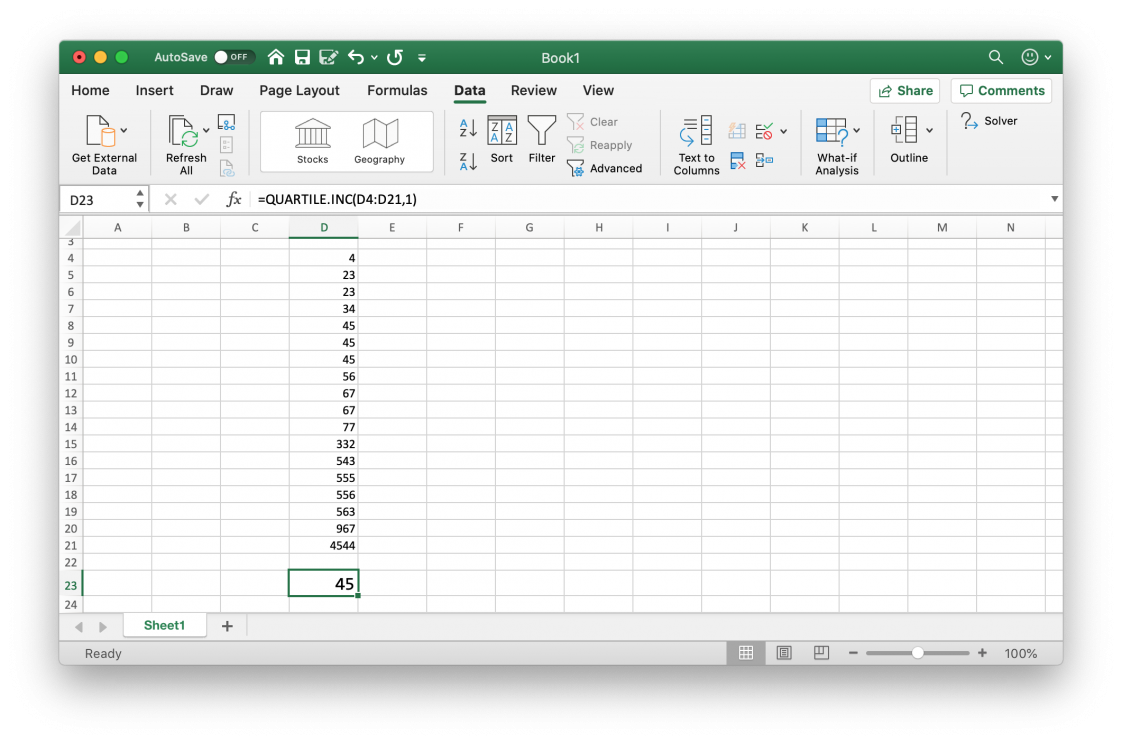
Excel quartile
Similar to the PERCENTILE formula, MS Excel has two functions that enable you to find the value in a range of numbers at a specific quartile.
QUARTILE.EXC is used if you want to obtain the quartile excluding the first and last values of the range (or array).
Conversely, QUARTILE.INC includes the first and last values of the range.
If you are interested in obtaining the value at the 2nd quartile, the formula is:
=QUARTILE.INC(start_of_range:end_of_range,2)Which is the same as the 50th percentile.
-

Excel percentile
MS Excel has two functions that enable you to find the value in a range of numbers at a specific percentile.
PERCENTILE.EXC is used if you want to obtain the percentile excluding the first and last values of the range (or array).
Conversely, PERCENTILE.INC includes the first and last values of the range.
So, you are interested in obtaining the value at the 25th percentile. The syntax for this is:
=PERCENTILE.INC(start_of_range:end_of_range,.25)The 50th percentile is:
=PERCENTILE.INC(start_of_range:end_of_range,.50)And the 75th percentile is:
=PERCENTILE.INC(start_of_range:end_of_range,.75) -
Statistics quantiles
Quantiles are useful for talking about where a particular value lies within a dataset. Unfortunately, they are not that widely understood.
We can think of quantile as equal portions of the data distribution. Once we have ordered the data, we can then split it up into different parts (tiles).
The first quarter of the data is referred to as the first quartile.
If we add another 25% of the data to the first quartile, we get the second quartile.
The third quartile contains the first 75% of the ordered data.
We can subtract the second quartile from the third quartile to find the interquartile range. This is the central 50% of the distribution.

Sometimes you will hear percentile or decile used when describing data. The percentile represents the proportion of the data that lies beneath an observed value. So, the 50th percentile is the values below which 50% of the data lies. Similarly, the 10th percentile represents 10% of the data.
The first quartile lies at the 25th percentile, the second quartile at 50% and the third quartile at 75%.
-

Excel: dealing with outliers
It has been said before, but having clean data is one of the best ways to ensure that your analysis is based on a sound footing.
In the same way that we can tell whether a picture hanging on the wall is a bit out of level, we can often recognise things in data that don’t seem to be quite correct. If we see a value that is much greater, or smaller than most of the other values in the sample, we might start to think that there was something amiss.
The challenge is that when we are looking at very large datasets, we cannot observe the outliers very easily. We might miss them altogether.
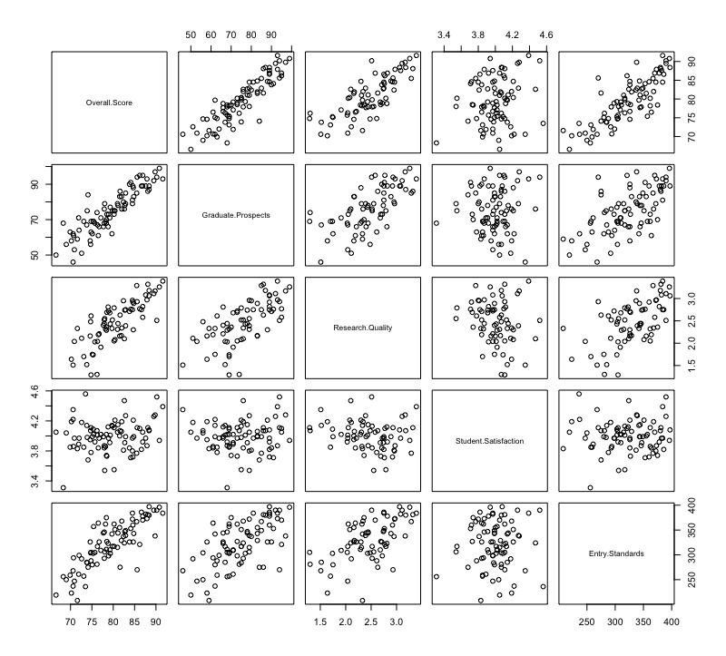
One approach is to visualise the data as a scatter plot for example, to see whether there are any outliers. Alternatively we can use our trusty spreadsheet to help us find the strange data.
In MS Excel, the MAX function locates the largest value from a range as follows:
=MAX(start_of_range, end_of_range)Conversely, the MIN function does the opposite:
=MIN(start_of_range, end_of_range)These two functions can be a great help when we are doing the initial checks of data that has been collected from an IIoT device.
-

Machine learning basics
Machine Learning (ML) is very popular at present. It’s capabilities are almost magical if you listen to the software vendors. There is no doubt that ML enables interesting capabilities. If you have ever browsed Amazon while being logged into your account, you will have witnessed the uncanny recommendations that it makes to entice you to make a purchase. These recommendations are based upon your historical interactions with the site; not only your purchase history, but the products that you have looked at, but not bought, as well.
ML has at its core a mathematical model, that enables predictions to be made about the future. However, this model is not static. Similar to humans, the mathematical model can be updated based upon new data that is fed into the model, and this is how retail websites such as Amazon can apparently track your buying and browsing patterns, and then recommend new products that appear to match your current interests.
The more data that is fed into a model, the more accurate the predictions become. ML can, in some cases, even generate predictions where there is no evidence of a particular situation existing within the model. This is where ML can appear to be ‘magical’.
Categorising Machine Learning
There are three categories of ML:
- Supervised learning – examples of known scenarios, with inputs and outcomes, are used to create the mathematical model. We can then use the model to either classify a future situation (place it into a known category, or we can use regression to deduce the relative strength of a relationship between an dependent variable and one ore more independent variables;
- Unsupervised learning – this is where the alchemy appears: patterns are observed without feeding the model with any known relationships between inputs and outcomes. Clustering is one example of technique used for unsupervised learning;
- Reinforcement learning – this refers to a mechanism whereby the process of ML is reinforced by positive or negative feedback from the environment. This operational data enriches the creation of the unsupervised model.
In practice, different ML approaches are combined to suit a particular domain problem. We might use unsupervised learning to simplify the problem domain when we don’t have a clear way forward. Once we have identified some patterns we can use these with a supervised learning technique. Or, for a domain that we know, we might create a supervised ML model, which is then refined by reinforcement learning.
-

Excel: mean, median, mode
A lot of people will use Microsoft Excel to do their analysis as it is installed on their desktop computer. To do basic descriptive statistics you will need to know how to calculate the mean, median and mode.
Mean
To calculate the mean requires the AVERAGE function as follows:
=AVERAGE(cell_ref1:cell_ref2)For example:
=AVERAGE(B2:B12)Calculates the mean of the values contained in the range B2 to B12.
Median
The median refers to the central value of a set of values:
=MEDIAN(cell_ref1:cell_ref2)If an even number of values is supplied to the MEDIAN function, the result will be calculated by taking the mean of the middle two values; this ensures that half of the data set is above the median value, and half of the dataset is below the median.
Mode
We use the MODE function when we want to find the most frequently occurring value.
=MODE(cell_ref1:cell_ref2) -
Fundamental statistics: average and standard deviation
This is the first of a series of posts where I explain some basic concepts for analytics. Fundamental statistics: average and standard deviation in particular, are important to understand. Especially, since statistics has a reputation for being a) complicated, b) boring, or c) both complicated and boring.
Having an understanding of statistics is useful and quite straightforward. If you take the trouble to find out what these essential concepts are, you’ll already be ahead of most people…
One misconception is that statistics is all about predicting the future, or forecasting, using bizarre mathematical equations. It is possible to use statistics for forecasting, and that is referred to as inferential statistics – we use some data to infer a future outcome.
Descriptive statistics
When we have some data to analyse, for example for a report, we use descriptive statistics.
One common example of a descriptive statistic is average. We use averages to get a sense of a ‘typical’ value when there is a set of values to choose from. This is typically the mean of a set of numbers (all the values summed together, and then divided by the total number of values in the sample).
It could be the median (the central value of a ranked set of values), or the mode (the value that occurs most frequently in a set).
If we have some temperature data from an industrial process, we might want to take the mean of that data to see what the general temperature is over a period of time.
If we calculated the median of the temperature data, we would be looking for the central value.
Why might that be important?
If the data has a few values that are much higher than the rest (perhaps a tool went blunt and the cutting temperature increased rapidly), the high values would actually inflate the mean. This would distort our view of the rest of the data. In such a case, the median is appropriate.
If we are interested in the most common temperature value – when the process has reached operating conditions for instance – then the mode is the average we are seeking.
Statistics ninja: standard deviation
However, if there is one term that separates those-who-know from those-who-don’t-know, it is standard deviation.
The standard deviation is a measure of how far the values in a data set are spread out. If the standard deviation is high, the values are further away from the mean. This is represented by a flat distribution. Conversely, a low standard deviation means that the values are close to the mean, so the dispersion is less. How is this useful?
When we are monitoring real-life processes, the data is not all neat and tidy. There are natural variations in the values that are recorded. Looking at such data, we need to be able to observe which values are acceptable. Those that are outside some arbitrary limits are referred to as outliers.
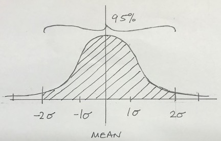
If the process temperature mean is 52 degrees celsius, with a standard deviation of 2 degrees we can say that:
- 1 standard deviation would represent 50 degrees to 54 degrees. This range accounts for 68.3% of the total distribution of values;

- 2 standard deviations is all of the values between 48 degrees and 56 degrees, which is 95.4% of the distribution;

- 3 standard deviations is virtually all of the values – 99.7%.

Applying the knowledge
One practical example of descriptive statistics in manufacturing is Lean Six Sigma. The Greek lower case symbol for standard deviation is sigma; as we have seen above, six of the standard deviations represents 99.7% of the values that are either side of the mean.
Six sigma is therefore a powerful concept when analysing process data.
Comprehending these fundamental statistical concepts is the key to getting the most out of IIoT implementations. Initially it may be about producing reports that are meaningful and aid your understanding of the process that you are monitoring.
The next stage is to have your Industrial Internet of Things devices produce not only the data, but also real-time descriptive statistics. Such statistics can then be used as the basis of triggers or alerts to intervene, which might support quality assurance for example.
Fundamental statistics: understanding the average and standard deviation of a dataset, is really important if you want to discover valuable insight.
If your reporting applications already do this, then at least you can understand how the data is being reported, and that will help you think about the opportunities to use data from more than one process to inform your decisions.
-

IIoT: Technical vs. people skills
You want your factory to be IIoT enabled. You’ve seen the videos and read the case studies. It’s obvious: IIoT technologies are central to your digital transformation.
But where do you start? How do you start?
The technologies of IIoT implicitly demand people with technical skills. While we travel through an early adoption phase, some plant can produce the data we need, but we’ll probably have to augment other plant so that it can do the same.
IIoT lends itself to the technophiles; even though the barriers to entry are lowering, if you want to fasten a data reporting capability onto a machine tool, you’ll need to know what you are doing.
If we consider the area where IIoT is flourishing currently – condition monitoring and predictive maintenance – then the domain is populated by technical people, with technical skills, doing technical things.
Some installations are moving to a service-oriented model, where the manufacturer does not get involved with the IIoT at all. The IIoT installer takes care of data monitoring, analytics, reporting and communication, and merely produces processed data to be consumed by the client.
If we want to transform a factory, we shall need to think much more broadly than a predictive maintenance solution. The complex interplay of multiple machines, material handling equipment, finishing plant, assembly lines, etc., suggests that there will be an imperative for the rapid up-skilling of existing staff to become more technical.
But we know that technology projects often fail when the focus is on the technology itself. Of course, it is the potential of the technology that justified the transformation project in the first place; however, people are still central to the operations and they need to be brought along with the change if the change is to stick.
So, IIoT implementation initiatives need a people-centric approach to lead the development of people-skills. Lean is a good way of approaching IIoT adoption as it focuses on the principles of efficiency, supporting the development of appropriate behaviours.
With such behaviours in place, IIoT can be `relegated’ to a technology that serves what people really need.